File:2014 militrary expenditures absolute.svg

此SVG文件的PNG预览的大小:512 × 288像素。 其他分辨率:320 × 180像素 | 640 × 360像素 | 1,024 × 576像素 | 1,280 × 720像素 | 2,560 × 1,440像素。
原始文件 (SVG文件,尺寸为512 × 288像素,文件大小:1.52 MB)
摘要
| 描述 |
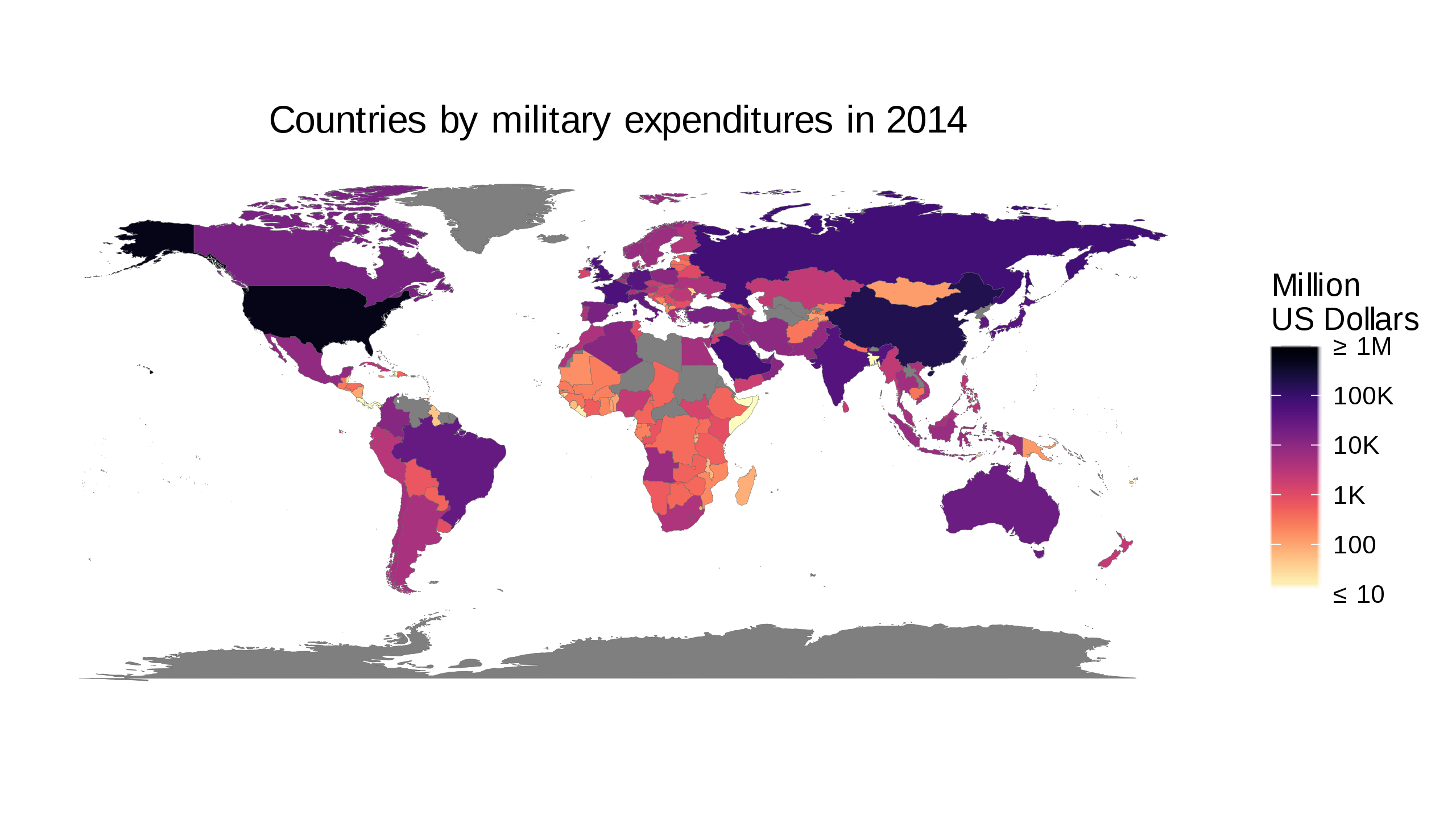
English: Based on the Worldbank data from http://data.worldbank.org/indicator/MS.MIL.XPND.GD.ZS and http://data.worldbank.org/indicator/NY.GDP.MKTP.CD This is a candidate for replacing/augmenting https://commons.wikimedia.org/wiki/File:Countries_by_Military_expenditures_(%25_of_GDP)_in_2014_v2.svg |
| 来源 | 自己的作品 |
| 作者 | Pipping |
_in_2014_v2.svg)
许可协议
我,本作品著作权人,特此采用以下许可协议发表本作品:
本文件采用知识共享署名-相同方式共享 4.0 国际许可协议授权。
- 您可以自由地:
- 共享 – 复制、发行并传播本作品
- 修改 – 改编作品
- 惟须遵守下列条件:
- 署名 – 您必须对作品进行署名,提供授权条款的链接,并说明是否对原始内容进行了更改。您可以用任何合理的方式来署名,但不得以任何方式表明许可人认可您或您的使用。
- 相同方式共享 – 如果您再混合、转换或者基于本作品进行创作,您必须以与原先许可协议相同或相兼容的许可协议分发您贡献的作品。
Created with the following piece of code:
library(magrittr)

selectedYear <- 2014

getWorldBankData <- function(indicatorCode, indicatorName) {
    baseName <- paste('API', indicatorCode, 'DS2_en_csv_v2', sep='_')
    ## Download zipfile if necessary
    zipfile <- paste(baseName, 'zip', sep='.')
    if (!file.exists(zipfile)) {
        zipurl <- paste(paste('http://api.worldbank.org/v2/en/indicator',
                              indicatorCode, sep='/'),
                        'downloadformat=csv', sep='?')
        download.file(zipurl, zipfile)
    }
    csvfile <- paste(baseName, 'csv', sep='.')
    ## This produces a warning because of the trailing commas. Safe to ignore.
    readr::read_csv(unz(zipfile, csvfile), skip=4,
                    col_types = list(`Indicator Name` = readr::col_character(),
                                     `Indicator Code` = readr::col_character(),
                                     `Country Name` = readr::col_character(),
                                     `Country Code` = readr::col_character(),
                                     .default = readr::col_double())) %>%
        dplyr::select(-c(`Indicator Name`, `Indicator Code`, `Country Name`))
}

## Obtain and merge World Bank data
worldBankData <-
    dplyr::left_join(
               getWorldBankData('MS.MIL.XPND.GD.ZS') %>%
               tidyr::gather(-`Country Code`, convert=TRUE,
                             key='Year', value=`Military expenditure (% of GDP)`,
                             na.rm = TRUE),
               getWorldBankData('NY.GDP.MKTP.CD') %>%
               tidyr::gather(-`Country Code`, convert=TRUE,
                             key='Year', value=`GDP (current US$)`,
                             na.rm = TRUE)) %>%
    dplyr::mutate(`Military expenditure (current $US)` =
                      `Military expenditure (% of GDP)`*`GDP (current US$)`/100) %>%
    dplyr::filter(Year == selectedYear) %>%
    dplyr::mutate(Year = NULL)

## Plotting: Obtain Geographic data
mapData <- tibble::as.tibble(ggplot2::map_data("world")) %>%
    dplyr::mutate(`Country Code` =
                      countrycode::countrycode(region, "country.name", "iso3c"),
                  ## This produces a warning but I do not see how we could do better
                  ## since we started with fuzzy names.
                  region = NULL, subregion = NULL)

combinedData <- dplyr::left_join(mapData, worldBankData)

## The default out-of-bounds function `censor` replaces values outside
## the range with NA. Since we have properly labelled the legend, we can
## project them onto the boundary instead
clamp <- function(x, range = c(0, 1)) {
    lower <- range[1]
    upper <- range[2]
    ifelse(x > lower, ifelse(x < upper, x, upper), lower)
}

ggplot2::ggplot(data = combinedData, ggplot2::aes(long,lat)) +
    ggplot2::geom_polygon(ggplot2::aes(group = group,
                                       fill  = `Military expenditure (current $US)`),
                          color = '#606060', lwd=0.05) +
    ggplot2::scale_fill_gradientn(colours= rev(viridis::magma(256, alpha = 0.5)),
                                  name   = "Million\nUS Dollars",
                                  trans  = "log",
                                  oob    = clamp,
                                  breaks = c(1e7,1e8,1e9,1e10,1e11,1e12),
                                  labels = c('\u2264 10', '100', '1K',
                                             '10K', '100K', '\u2265 1M'),
                                  limits = c(1e7,1e12)) +
    ggplot2::coord_fixed() +
    ggplot2::theme_bw() +
    ggplot2::theme(plot.title = ggplot2::element_text(hjust = 0.5),
          axis.title = ggplot2::element_blank(),
          axis.text = ggplot2::element_blank(),
          axis.ticks = ggplot2::element_blank(),
          panel.grid.major = ggplot2::element_blank(),
          panel.grid.minor = ggplot2::element_blank(),
          panel.border = ggplot2::element_blank(),
          panel.background = ggplot2::element_blank()) +
    ggplot2::labs(title = paste("Countries by military expenditures in",
                                selectedYear))

ggplot2::ggsave(paste(selectedYear, 'militrary_expenditures_absolute.svg', sep='_'),
                height=100, units='mm')
文件历史
点击某个日期/时间查看对应时刻的文件。
| 日期/时间 | 缩略图 | 大小 | 用户 | 备注 | |
|---|---|---|---|---|---|
| 当前 | 2017年5月20日 (六) 14:30 | | 512 × 288(1.52 MB) | Pipping | redo with dplyr |
| 2017年5月13日 (六) 12:12 |  | 512 × 256(1.51 MB) | Pipping | Handle truncation of the data range better: We distinguish between 0 and no data, but any existing datum below 10M USD is coloured the same way and all data above 1T USD are coloured the same way. The legend makes this clear. | |
| 2017年5月13日 (六) 08:55 |  | 512 × 256(1.51 MB) | Pipping | Completely redone. The former was in local currency (so that comparisons from country to country made absolutely no sense). Now everything is in current US dollars. | |
| 2017年5月11日 (四) 22:32 |  | 512 × 256(1.5 MB) | Pipping | Fixed min/max value for colors that kept anything below 1,000,000,000 US dollars from having a colour (now: Anything above 1,000,000 US dollars has a colour). | |
| 2017年5月11日 (四) 21:30 |  | 512 × 256(1.51 MB) | Pipping | {{Information |Description ={{en|1=English: Based on the Worldbank data from http://data.worldbank.org/indicator/MS.MIL.XPND.CN This is a candidate for replacing/augmenting https://commons.wikimedia.org/wiki/File:Countries_by_Military_expenditures_(... |
文件用途
没有页面使用本文件。
全域文件用途
以下其他wiki使用此文件:
- bg.wikipedia.org上的用途
- ca.wikipedia.org上的用途
- en.wikipedia.org上的用途
- eu.wikipedia.org上的用途
- sr.wikipedia.org上的用途
- th.wikipedia.org上的用途
- uk.wikipedia.org上的用途